Discovering Feature Circuits
Six landmark works that extract SAE and Transcoder features and link them into interpretable circuits via analytical attribution or patching.
Existing works in the feature circuit discovery domain first extract interpretable features using either Transcoder variants[Ameisen et al., 2025][Dunefsky et al., 2024][Ge et al., 2024] or Sparse Autoencoders.[Kissane et al., 2024][Ge et al., 2024][He et al., 2024][Marks et al., 2024] To link the extracted features into circuits, the dominant methodology is to define analytical feature edges (see §3). Only [Marks et al., 2024] utilizes patching.
Transcoder Feature Circuits
Dunefsky et al. (2024) — Transcoders Find Interpretable LLM Feature Circuits
Dunefsky et al. [2024] analyze the effectiveness of Transcoders in circuit discovery. Their work does not rely on using SAEs to interpret the attention layers. They simplify the attention module by only considering the OV circuitry with fixed attention scores. Thus, information flow within the attention module is analyzed, but not the information routing. The authors acknowledge this as a limitation, noting that the OV circuitry itself is highly informative.
Two types of feature interactions are considered: direct interaction (residual stream) and OV-mediated interaction. Their formulation of OV attribution is token-centric—it identifies which source tokens contribute most to a target feature through an attention head:
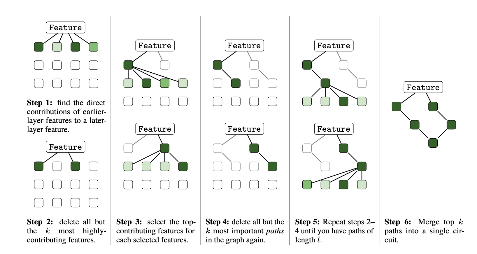
The subgraph discovery process begins with a target Transcoder feature \(b^{(j)}\). Earlier Transcoder features \(a^{(j)}\) that have high direct attribution to \(b^{(j)}\) are identified, and the process is recursed for those features. If an attention head shows high attribution, it is included in the circuit, and the search is recursed on the top-attributing token identified via the above equation. To do this, the downstream feature is passed back through the OV circuit to generate a new search vector at the source token:
This resulting vector is treated as a new search objective, and earlier features or attention heads that contributed to it are identified. The process is recursed again for those features and attention heads. Individual paths are then merged to form a single unified circuit.
Ameisen et al. (2025) — Circuit Tracing
Ameisen et al. [2025] replace the MLP layers with crosscoders (see §3) to construct an interpretable replacement model. Similar to [Dunefsky et al., 2024], a forward pass is performed to cache the active features and attention patterns, and only the OV circuit is analyzed while QK scores are treated as fixed.
By freezing the attention patterns and normalization denominators (effectively applying stop-gradients to all non-linearities), the replacement model is linearized with respect to the input. The active features are then linked using a method analogous to [Dunefsky et al., 2024], adapted to the crosscoder case. A feature in a crosscoder lives in (writes to) many layers simultaneously. The attribution from feature \(a\) (at token \(i\)) to feature \(b\) (at token \(j\)) is given by:
Summation runs over all layers \(\ell\) that feature \(a\) writes to (up to \(\ell_b\)). \(J_{i,\ell \to j,\ell_b}^{\nabla}\) is the Jacobian of the frozen residual stream, representing the linear transformation the feature vector undergoes as it propagates from layer \(\ell\) to layer \(\ell_b\). Since the frozen model is linear, this Jacobian equals the gradient of the target residual stream with respect to the source residual stream—enabling efficient computation via backpropagation.
The backward recursive circuit-forming procedure is largely similar to [Dunefsky et al., 2024]: start at an end feature to explain, identify the highest contributors, and recurse.
Kamath et al. (2025) — Tracing Attention Computation
Ameisen et al. [2025] note that the inability to explain attention patterns is a significant limitation, as these patterns are often the crux of model behavior. In their successor work, Kamath et al. [2025] address this by extending the method to explicitly trace attention computation.
The aggregated attribution in the crosscoder equation (above) makes it difficult to isolate the dominant attention head for a given feature-to-feature attribution, preventing us from tracing the routing logic. This becomes severe for features in distant layers, as the number of attention paths grows exponentially with depth.
The authors experimented with placing SAEs on attention outputs as checkpoints, but this resulted in high reconstruction errors and circuits dominated by error nodes. Their final approach places SAEs on the residual stream of every layer, so edges are strictly layer-wise. To then analyze the contribution of head \(h\) to an edge \((a \to b)\):
The total attribution for an edge \((a \to b)\) sums this term over all attention heads, plus contributions from the MLP and residual stream. In practice, the authors use Weakly Causal Cross Coders (WCCs)—similar to SAEs but reading from layer \(L\) and reconstructing residual streams at layers \(L, L+1, \dots, N\)—to capture linear propagation across layers. Once the dominant attention head for an edge is identified, the bilinear QK decomposition from §3 is used to explain the attention pattern itself (extended to account for RoPE, LayerNorms, and biases). Circuit construction follows the same backward iterative process as [Dunefsky et al., 2024].
Transcoders & SAEs — Ge et al. (2024)
Ge et al. [2024] obtain a linear computation graph of active SAE and Transcoder features resulting from an input, then prunes this graph to isolate the relevant circuit for a target output using a gradient-based method called Hierarchical Attribution.
Three types of feature interactions are analyzed:
- Type 1: Upstream feature \(a\) → Transcoder feature \(b\) (direct residual-stream contribution)
- Type 2: Upstream feature \(a^{(i)}\) → Attention Output (OV) feature \(b^{(j)}\)
- Type 3: Feature–feature resonance contributing to an attention score (QK circuit)
Circuit discovery starts with a forward pass where the active SAE/Transcoder features and QK scores are identified. Active features are linked using Type 1 and Type 2 edges, forming a graph that is then pruned with respect to a target output logit.
Pruning is attribution-based: an upstream node's gradient is computed as the sum of gradients back-propagated from its non-pruned successors. Its attribution is \(\text{gradient} \times \text{activation}\). If a node's attribution falls below a threshold, it is pruned. The graph is traversed breadth-first from the output, propagating pruning upstream.
Important attention scores are subsequently analyzed using Type 3 (QK attribution). Once important feature pairs for an interesting attention score are identified, those features are attributed through the upstream OV+Transcoder circuits (Type 2, then Type 1), iterating to obtain the full computation graph of the attention mechanism.
SAE Feature Circuits
He et al. (2024) — Dictionary Learning for Circuit Discovery
He et al. [2024] place SAEs on Embeddings, Attention outputs, and MLP outputs, and define three types of feature interactions:
- Upstream feature → Attention output feature (OV Circuit)
- Feature–feature resonance for an attention score (QK Circuit)
- Upstream feature → MLP output feature
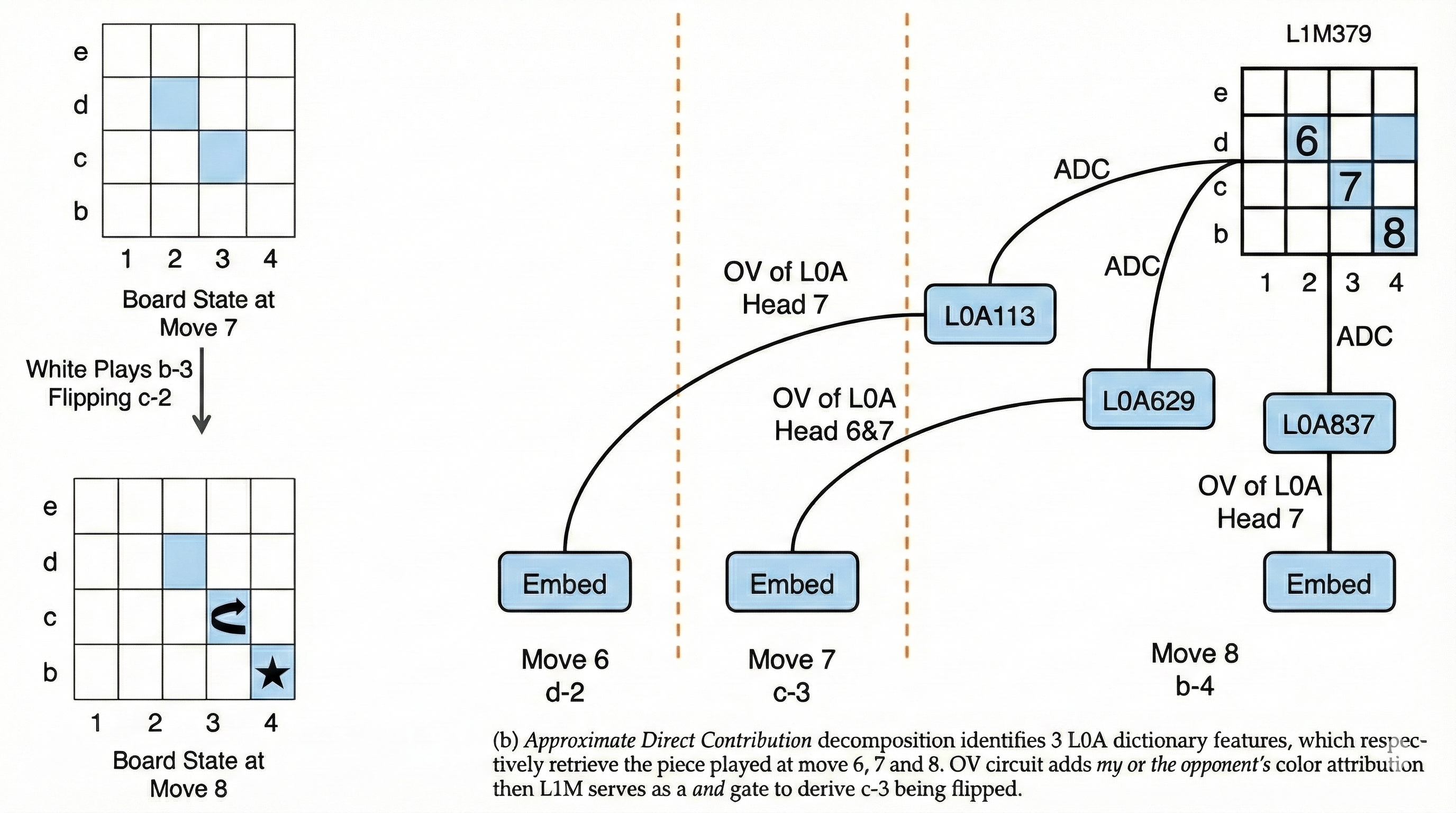
Because Transcoders are not used here, the MLP layer remains a non-linear operation. To resolve this, the authors introduce Approximate Direct Contribution (ADC), which linearizes the MLP for a specific input by freezing the activation states of ReLU (binary) and GeLU (slope):
where \(W_{\text{in}}\) and \(W_{\text{out}}\) are the MLP's internal weights and \(\sigma'\) represents the frozen activation states computed on the total input \(x_{\text{total}}\).
Circuit construction from a target feature is conducted top-down: using ADC or OV-circuitry, iterating over all attention heads, tokens, and active features. The top attributing upstream features are identified and the process is recursed. Crucially, if a top feature is mediated through an attention head, the feature pair responsible for routing the information flow (the attention score) is identified using the QK bilinear decomposition. The discovery process is also recursed on these "routing" features to understand the cause of the attention pattern itself.
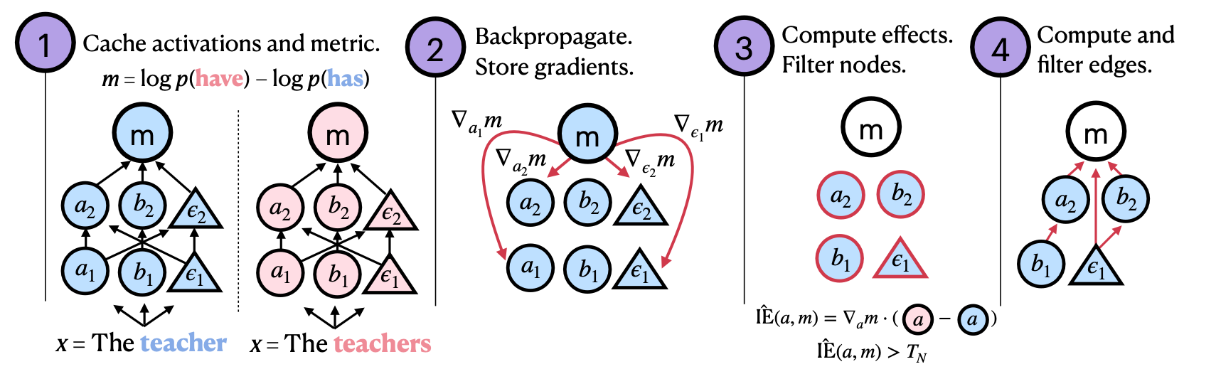
Marks et al. (2024) — Sparse Feature Circuits
Marks et al. [2024] place SAEs on attention and MLP outputs, as well as residual streams. Rather than relying on analytical edges, they use patching to filter nodes and edges. The nodes consist of the active SAE features for the given inputs.
The method performs attribution patching on these features to isolate those relevant to the computation of the target metric \(m\). Subsequently, edge patching is performed to quantify and filter the edges connecting the relevant features. This results in a sparse, interpretable subgraph—the feature circuit for the behavior of interest. Notably, this is the only surveyed method that relies on patching rather than closed-form analytical edges.