Core Methods

Sparse Autoencoders (SAEs)

Polysemantic neurons pose a significant challenge to interpretability research because neurons themselves are not interpretable causal units. We are interested in the monosemantic features that compose these polysemantic signals. However, it is not possible to naively decompose these signals, as the features are highly tangled.

Sparse Autoencoders (SAEs) were introduced to disentangle these polysemantic signals.[Cunningham et al., 2024] SAEs do not require modifying the original models; rather, they process the signal and decompose it into human-interpretable features.

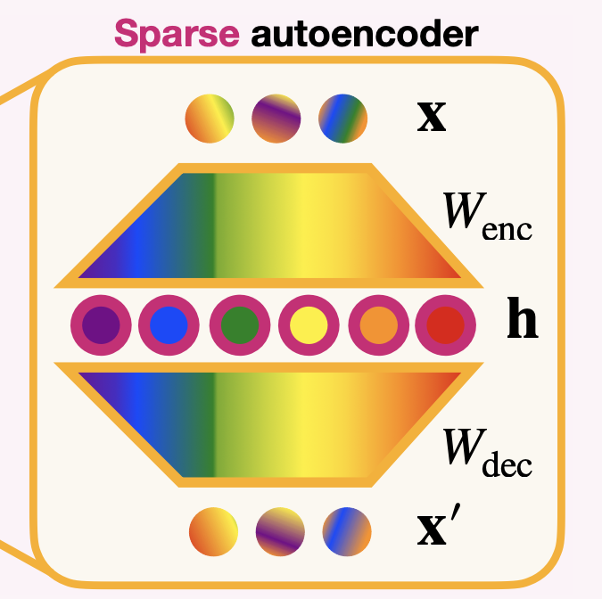
SAEs encode the input signal into a higher-dimensional hidden state using an encoder matrix \(W_{\text{enc}}\). They then reconstruct the input from this hidden state using a decoder matrix \(W_{\text{dec}}\). The autoencoder is trained to minimize the reconstruction error, adding an \(L_1\) penalty to enforce sparsity in the hidden state, ensuring that the hidden representations remain interpretable.

SAEs are typically placed at key locations in the residual stream—on embedding outputs, attention outputs, MLP outputs, or the residual stream itself between layers. Each placement yields a dictionary of features at that computational stage.

Transcoders

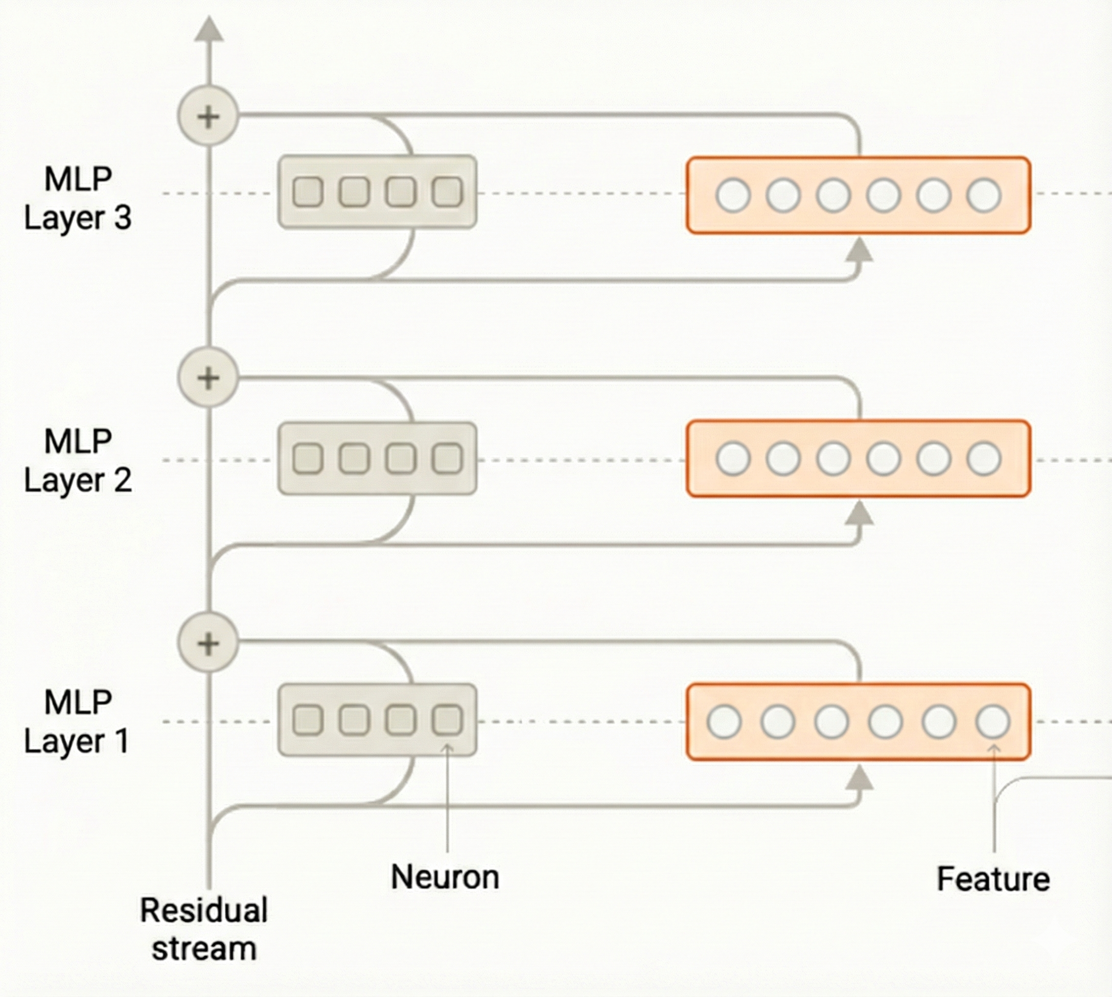
Transcoders were developed to interpret the computation of the MLP sublayer.[Dunefsky et al., 2024] They allow for the discovery of features involved in the MLP's transformation. Formally, a Transcoder is defined as:

where \(x\) is the input to the MLP sublayer. Crucially, the encoder width is chosen to be much larger than the original MLP's width. This allows the Transcoder to represent features explicitly without superposition, as they do not need to be compressed into a lower-dimensional space. Since the Transcoder is trained on the input–output pairs of the MLP, it serves as an interpretable approximation of the dense MLP sublayer.

Crosscoders

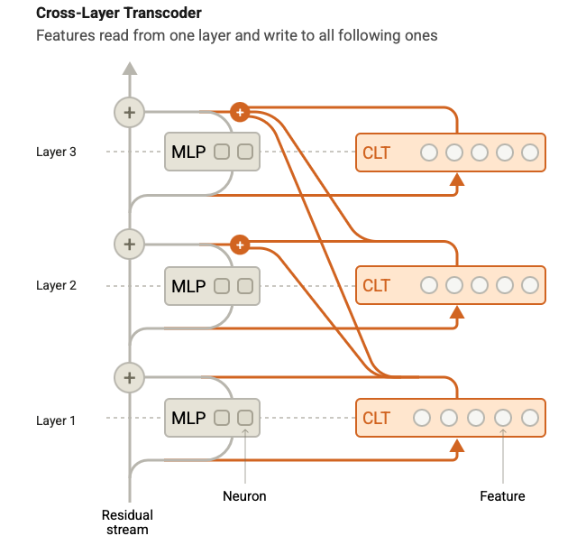
Crosscoders are introduced as an extension to Transcoders by[Ameisen et al., 2025]. Essentially, Crosscoders are cross-layer Transcoders: a crosscoder reads from its layer's residual stream but writes to the reconstruction targets of all subsequent layers. The motivation behind this approach is to prevent the re-discovery of certain features, as regular Transcoders end up re-discovering identical features across layers. When the Layer 1 crosscoder learns a feature, it writes that feature to the output of all other layers, so the remaining crosscoders need not re-discover it. This simplifies the discovered circuits.

Analytical Feature Edges

The works that utilize analytical edge weights to construct feature circuits describe similar methods, grounded in the linear structure shared by SAEs and Transcoders.

Note that both SAEs and Transcoders have essentially identical structures—an encoder and a decoder. They differ primarily in their training objective: SAEs reconstruct their input (input → input), whereas Transcoders approximate a sub-module's function (MLP input → MLP output).

A feature residing inside an SAE or Transcoder is written to the residual stream by multiplying its scalar activation value with its decoder vector, effectively transforming the feature into residual-stream space. Conversely, a feature's activation is computed by projecting the residual stream onto its encoder vector (followed by a non-linearity). Notice that if feature \(a\)'s decoder and feature \(b\)'s encoder align, these two features share a strong edge: when \(a\) fires, it strongly contributes to firing \(b\).

Direct Attribution

This measures the direct contribution of an upstream feature \(a\) to a downstream feature \(b\) at the same token through the residual stream:

Attention Attribution

Following[Elhage et al., 2021], the Attention mechanism consists of two independent circuits: the QK circuit and the OV circuit. If the QK scores (attention scores) are treated as fixed, the attention mechanism is functionally described by the OV circuit, where QK scores act as scalar scaling factors. For a fixed pattern, attention becomes a linear transformation of the residual stream defined by \(W_{OV} = W_O W_V\).

OV Circuit Attribution

The contribution of feature \(a\) (at token \(i\)) to feature \(b\) (at token \(j\)), mediated by the OV circuit of a specific head, is:

This term captures what information is moved by the attention head, but not why it was moved, since it treats attention scores as fixed constants.

QK Circuit Attribution

To understand the composition of the attention pattern itself, we look at the QK circuit. The contribution of feature \(a\) (active at token \(i\), the Query) and feature \(b\) (active at token \(j\), the Key) to the attention score is:

This term captures the "resonance" between feature \(a\) in the query position and feature \(b\) in the key position, determining how strongly the head attends to token \(j\) given these specific features.

Patching

Patching is a well-established method for analyzing a component's (e.g., a neuron or attention head) causal effect on a target metric, often a logit or another downstream component.

Zero Ablation

The simplest variant is zero patching, where the activation value of the component is manually set to zero and the effect on the logit is observed. However, this creates an Out-of-Distribution (OOD) problem: a neuron's natural activation is rarely exactly zero. This potentially breaks the computation rather than revealing causality.

Activation Patching

Activation patching addresses this by sourcing the intervention value from a natural input. The model is run with two inputs: a clean input and a corrupt input (e.g., a counterfactual prompt). We store the activations from both passes. Rather than zeroing out a clean component, we replace its activation with the corresponding value from the corrupt pass and observe the change in the target metric. Patching each component requires a separate forward pass, making it computationally infeasible for fine-grained analysis across large models.

Attribution Patching

To remedy this,[Syed et al., 2023] formalized Attribution Patching, originally proposed by[Nanda, 2023]. This technique approximates the effect of activation patching using a first-order Taylor expansion:

Here, \(\nabla_{a}\, m \big|_{a = a_{\text{clean}}}\) is the gradient of the task-specific metric with respect to the activation, calculated for all nodes simultaneously via a single backward pass. This eliminates the need for separate forward passes for every component. If a patched input is not available, \(a_{\text{patch}}\) is simply set to \(0\) for zero ablation.

Edge Patching

The attribution patching formulation for a node can be extended to the attribution of an edge. While the equation above captures the attribution of all paths originating from \(a\), we aim to isolate the contribution of the specific edge \(a \to b\):

Here, \(\nabla_{a,\, \text{stop}(\mathcal{M})}\, b \big|_{a_{\text{clean}}}\) is the gradient of the downstream node \(b\) with respect to the upstream node \(a\), computed by applying stop-gradients to all intermediate nodes \(\mathcal{M}\) during backpropagation. When multiplied by the gradient of the metric \(m\) with respect to \(b\), we obtain the gradient of the metric with respect to \(a\) mediated exclusively through the edge \(e_{a \to b}\).